// Index and parameter values.
data {
  int<lower = 1> N;    // Number of observations.
  int<lower = 1> I;    // Number of covariates.
  matrix[N, I] X;      // Matrix of covariates.

  vector[I] beta;      // Vector of slopes.
  real<lower = 0> tau; // Variance of the regression.
}

// Generate data according to the flat regression.
generated quantities {
  // Vector of observations.
  vector[N] y;

  // Generate data.
  for (n in 1:N) {
    y[n] = normal_rng(X[n,] * beta, tau);
  }
}There are a number of ways to code (i.e., encode) discrete (i.e., categorical) explanatory variables, with different coding strategies suited for specific use cases. In this post, we explore using two of the most common ways to code discrete explanatory variables: dummy coding and index coding. Another approach is called effects or sum-to-one coding. For a great walkthrough of that approach and its benefits in the context of choice modeling, see Elea Feit’s post that helped inspire this one.
Let’s start by generating flat regression data that includes discrete explanatory variables.
Now we create the matrix of covariates and call generate_flat_regression_data.
# Load packages.
library(tidyverse)
library(cmdstanr)
library(posterior)
library(bayesplot)
library(tidybayes)

# Set the simulation seed.
set.seed(42)

# Specify data and parameter values.
sim_values <- list(
  N = 50,                    # Number of observations.
  I = 5,                     # Number of covariates.
  J = c(2, 3),               # Number of levels for each discrete variable.
  beta = c(1, -4, 6, 3, -2), # Vector of slopes.
  tau = 1                    # Variance of the regression.
)

# Matrix of covariates.
sim_X <- matrix(data = 0, nrow = sim_values$N, ncol = (sim_values$I))
for (n in 1:sim_values$N) {
  temp_X <- NULL
  for (j in 1:length(sim_values$J)) {
    temp_J <- rep(0, sim_values$J[j])
    temp_J[sample(seq(1, (sim_values$J[j])), 1)] <- 1
    temp_X <- c(temp_X, temp_J)
  }
  sim_X[n,] <- temp_X
}
sim_values$X <- sim_X

head(sim_values$X)
[,1] [,2] [,3] [,4] [,5]
[1,] 1 0 1 0 0
[2,] 1 0 1 0 0
[3,] 0 1 0 1 0
[4,] 0 1 1 0 0
[5,] 0 1 0 0 1
[6,] 0 1 0 0 1# Compile the model for generating data.
generate_flat_regression_data <- cmdstan_model(
stan_file = here::here("posts", "discrete-coding", "Code", "generate_flat_regression_data.stan"),
dir = here::here("posts", "discrete-coding", "Code", "Compiled")
)
# Generate data.
sim_data <- generate_flat_regression_data$sample(
data = sim_values,
chains = 1,
iter_sampling = 1,
seed = 42,
fixed_param = TRUE
)Running MCMC with 1 chain...
Chain 1 Iteration: 1 / 1 [100%] (Sampling)
Chain 1 finished in 0.0 seconds.# Extract generated data.
sim_y <- sim_data$draws(variables = "y", format = "draws_list") %>%
pluck(1) %>%
flatten_dbl()
head(sim_y)[1] 6.927270 8.074890 -0.379599 2.647710 -4.816130 -5.506060Dummy coding
Also known as indicator coding, dummy coding is the most common way to deal with discrete variables, where a single discrete variable with K levels is encoded as K - 1 binary columns, each indicating the presence or absence of the given level. It is an approach to identifying the estimates of discrete explanatory levels that has a specific contrast hard-wired.
If we include all levels of a single discrete variable, they sum up across columns to a constant—to an intercept. If we did that with more than one discrete variable, we would have more than one intercept and they would no longer be identified. With dummy coding, it is typical to include an intercept (i.e., a constant, often a column of 1’s) and drop the first level (i.e., the reference level) of each of the discrete variables.
Here’s a flat regression using dummy coding.
// Index value and observations.
data {
  int<lower = 1> N;    // Number of observations.
  int<lower = 1> I;    // Number of covariates.
  vector[N] y;         // Vector of observations.
  matrix[N, I] X;      // Matrix of covariates.
}

// Parameters.
parameters {
  real alpha;          // Intercept.
  vector[I] beta;      // Vector of slopes.
  real<lower = 0> tau; // Variance of the regression.
}

// Regression.
model {
  // Priors.
  alpha ~ normal(0, 5);
  for (i in 1:I) {
    beta[i] ~ normal(0, 5);
  }
  tau ~ normal(0, 5);

  // Likelihood.
  for (n in 1:N) {
    y[n] ~ normal(alpha + X[n,] * beta, tau);
  }
}
Let’s run this flat regression using dummy coding.
# Specify data.
data <- list(
  N = length(sim_y),    # Number of observations.
  I = ncol(sim_X) - 2,  # Number of covariates.
  y = sim_y,            # Vector of observations.
  X = sim_X[, -c(1, 3)] # Matrix of covariates.
)

# Compile the model.
flat_regression_dummy <- cmdstan_model(
  stan_file = here::here("posts", "discrete-coding", "Code", "flat_regression_dummy.stan"),
  dir = here::here("posts", "discrete-coding", "Code", "Compiled")
)

# Fit the model.
fit_dummy <- flat_regression_dummy$sample(
  data = data,
  chains = 4,
  parallel_chains = 4,
  seed = 42
)
Running MCMC with 4 parallel chains...
Chain 1 Iteration: 1 / 2000 [ 0%] (Warmup)
Chain 1 Iteration: 100 / 2000 [ 5%] (Warmup)
Chain 1 Iteration: 200 / 2000 [ 10%] (Warmup)
Chain 1 Iteration: 300 / 2000 [ 15%] (Warmup)
Chain 1 Iteration: 400 / 2000 [ 20%] (Warmup)
Chain 1 Iteration: 500 / 2000 [ 25%] (Warmup)
Chain 1 Iteration: 600 / 2000 [ 30%] (Warmup)
Chain 1 Iteration: 700 / 2000 [ 35%] (Warmup)
Chain 1 Iteration: 800 / 2000 [ 40%] (Warmup)
Chain 1 Iteration: 900 / 2000 [ 45%] (Warmup)
Chain 1 Iteration: 1000 / 2000 [ 50%] (Warmup)
Chain 1 Iteration: 1001 / 2000 [ 50%] (Sampling)
Chain 1 Iteration: 1100 / 2000 [ 55%] (Sampling)
Chain 1 Iteration: 1200 / 2000 [ 60%] (Sampling)
Chain 1 Iteration: 1300 / 2000 [ 65%] (Sampling)
Chain 1 Iteration: 1400 / 2000 [ 70%] (Sampling)
Chain 1 Iteration: 1500 / 2000 [ 75%] (Sampling)
Chain 1 Iteration: 1600 / 2000 [ 80%] (Sampling)
Chain 1 Iteration: 1700 / 2000 [ 85%] (Sampling)
Chain 1 Iteration: 1800 / 2000 [ 90%] (Sampling)
Chain 1 Iteration: 1900 / 2000 [ 95%] (Sampling)
Chain 1 Iteration: 2000 / 2000 [100%] (Sampling)
Chain 2 Iteration: 1 / 2000 [ 0%] (Warmup)
Chain 2 Iteration: 100 / 2000 [ 5%] (Warmup)
Chain 2 Iteration: 200 / 2000 [ 10%] (Warmup)
Chain 2 Iteration: 300 / 2000 [ 15%] (Warmup)
Chain 2 Iteration: 400 / 2000 [ 20%] (Warmup)
Chain 2 Iteration: 500 / 2000 [ 25%] (Warmup)
Chain 2 Iteration: 600 / 2000 [ 30%] (Warmup)
Chain 2 Iteration: 700 / 2000 [ 35%] (Warmup)
Chain 2 Iteration: 800 / 2000 [ 40%] (Warmup)
Chain 2 Iteration: 900 / 2000 [ 45%] (Warmup)
Chain 2 Iteration: 1000 / 2000 [ 50%] (Warmup)
Chain 2 Iteration: 1001 / 2000 [ 50%] (Sampling)
Chain 2 Iteration: 1100 / 2000 [ 55%] (Sampling)
Chain 2 Iteration: 1200 / 2000 [ 60%] (Sampling)
Chain 2 Iteration: 1300 / 2000 [ 65%] (Sampling)
Chain 2 Iteration: 1400 / 2000 [ 70%] (Sampling)
Chain 2 Iteration: 1500 / 2000 [ 75%] (Sampling)
Chain 2 Iteration: 1600 / 2000 [ 80%] (Sampling)
Chain 2 Iteration: 1700 / 2000 [ 85%] (Sampling)
Chain 2 Iteration: 1800 / 2000 [ 90%] (Sampling)
Chain 2 Iteration: 1900 / 2000 [ 95%] (Sampling)
Chain 2 Iteration: 2000 / 2000 [100%] (Sampling)
Chain 3 Iteration: 1 / 2000 [ 0%] (Warmup)
Chain 3 Iteration: 100 / 2000 [ 5%] (Warmup)
Chain 3 Iteration: 200 / 2000 [ 10%] (Warmup)
Chain 3 Iteration: 300 / 2000 [ 15%] (Warmup)
Chain 3 Iteration: 400 / 2000 [ 20%] (Warmup)
Chain 3 Iteration: 500 / 2000 [ 25%] (Warmup)
Chain 3 Iteration: 600 / 2000 [ 30%] (Warmup)
Chain 3 Iteration: 700 / 2000 [ 35%] (Warmup)
Chain 3 Iteration: 800 / 2000 [ 40%] (Warmup)
Chain 3 Iteration: 900 / 2000 [ 45%] (Warmup)
Chain 3 Iteration: 1000 / 2000 [ 50%] (Warmup)
Chain 3 Iteration: 1001 / 2000 [ 50%] (Sampling)
Chain 3 Iteration: 1100 / 2000 [ 55%] (Sampling)
Chain 3 Iteration: 1200 / 2000 [ 60%] (Sampling)
Chain 3 Iteration: 1300 / 2000 [ 65%] (Sampling)
Chain 3 Iteration: 1400 / 2000 [ 70%] (Sampling)
Chain 3 Iteration: 1500 / 2000 [ 75%] (Sampling)
Chain 3 Iteration: 1600 / 2000 [ 80%] (Sampling)
Chain 3 Iteration: 1700 / 2000 [ 85%] (Sampling)
Chain 3 Iteration: 1800 / 2000 [ 90%] (Sampling)
Chain 3 Iteration: 1900 / 2000 [ 95%] (Sampling)
Chain 3 Iteration: 2000 / 2000 [100%] (Sampling)
Chain 4 Iteration: 1 / 2000 [ 0%] (Warmup)
Chain 4 Iteration: 100 / 2000 [ 5%] (Warmup)
Chain 4 Iteration: 200 / 2000 [ 10%] (Warmup)
Chain 4 Iteration: 300 / 2000 [ 15%] (Warmup)
Chain 4 Iteration: 400 / 2000 [ 20%] (Warmup)
Chain 4 Iteration: 500 / 2000 [ 25%] (Warmup)
Chain 4 Iteration: 600 / 2000 [ 30%] (Warmup)
Chain 4 Iteration: 700 / 2000 [ 35%] (Warmup)
Chain 4 Iteration: 800 / 2000 [ 40%] (Warmup)
Chain 4 Iteration: 900 / 2000 [ 45%] (Warmup)
Chain 4 Iteration: 1000 / 2000 [ 50%] (Warmup)
Chain 4 Iteration: 1001 / 2000 [ 50%] (Sampling)
Chain 4 Iteration: 1100 / 2000 [ 55%] (Sampling)
Chain 4 Iteration: 1200 / 2000 [ 60%] (Sampling)
Chain 4 Iteration: 1300 / 2000 [ 65%] (Sampling)
Chain 4 Iteration: 1400 / 2000 [ 70%] (Sampling)
Chain 4 Iteration: 1500 / 2000 [ 75%] (Sampling)
Chain 4 Iteration: 1600 / 2000 [ 80%] (Sampling)
Chain 4 Iteration: 1700 / 2000 [ 85%] (Sampling)
Chain 4 Iteration: 1800 / 2000 [ 90%] (Sampling)
Chain 4 Iteration: 1900 / 2000 [ 95%] (Sampling)
Chain 4 Iteration: 2000 / 2000 [100%] (Sampling)
Chain 1 finished in 0.1 seconds.
Chain 2 finished in 0.1 seconds.
Chain 3 finished in 0.1 seconds.
Chain 4 finished in 0.1 seconds.
All 4 chains finished successfully.
Mean chain execution time: 0.1 seconds.
Total execution time: 0.2 seconds.Note that we can’t directly recover the parameters values we used when simulating the data. Dummy coding is equivalent to specifying each included level as a “hard-wired” contrast with the reference level. We can compare the dummy-coded marginal posteriors to the contrasted true parameter values.
# Extract draws and compare contrasts.
contrast_values <- tibble(
  .variable = str_c("contrast", 1:(sim_values$I - length(sim_values$J))),
  values = c(
    # First discrete variable.
    sim_values$beta[2] - sim_values$beta[1],
    # Second discrete variable.
    sim_values$beta[4] - sim_values$beta[3],
    sim_values$beta[5] - sim_values$beta[3]
  )
)
fit_dummy$draws(variables = "beta", format = "draws_df") %>%
  mutate_variables(
    contrast1 = `beta[1]`,
    contrast2 = `beta[2]`,
    contrast3 = `beta[3]`
  ) %>%
  gather_draws(contrast1, contrast2, contrast3) %>%
  ggplot(aes(y = .variable, x = .value)) +
  stat_histinterval() +
  geom_vline(aes(xintercept = values), contrast_values, color = "red") +
  facet_wrap(~ .variable, scales = "free", ncol = 1)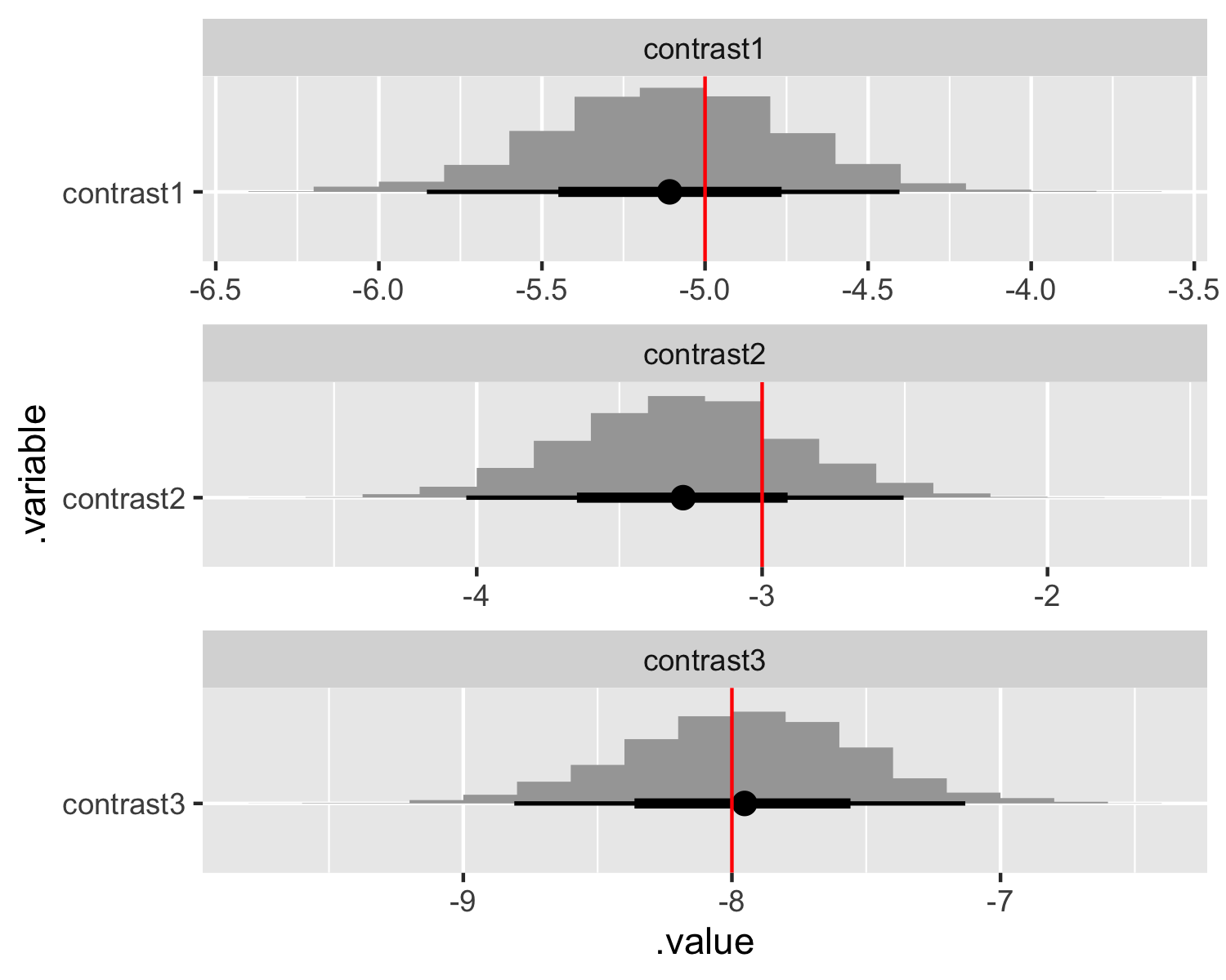
The drawback to dummy coding in a Bayesian setting with real data is that we need to specify priors over the contrasts rather than the parameters themselves. This complication for setting priors is a good reason to consider effects coding (again, see Elea Feit’s post on that topic). Dummy coding also enshrines the reference level as something special, making it non-trivial to compute other contrasts.
Index coding
Also known as one-hot encoding, index coding similarly turns each level of a discrete variable into its own binary column. However, with index coding we don’t include an intercept and don’t include any reference levels.
By not including reference levels, the intercept is implied by the fact that the columns sum to a constant, as discussed previously. But when we have more than one discrete variable we also have more than one implied intercept. This would create an identification problem in a frequentist setting, but in a Bayesian analysis we simply rely on the prior to enable identification of each of the parameters. As a bonus, the contrasts are always identified even if their constituent parameter estimates are not.
Here’s a flat regression using index coding. Note that the only difference here is the absence of the intercept alpha.
// Index value and observations.
data {
  int<lower = 1> N;    // Number of observations.
  int<lower = 1> I;    // Number of covariates.
  vector[N] y;         // Vector of observations.
  matrix[N, I] X;      // Matrix of covariates.
}

// Parameters.
parameters {
  vector[I] beta;      // Vector of slopes.
  real<lower = 0> tau; // Variance of the regression.
}

// Regression.
model {
  // Priors.
  for (i in 1:I) {
    beta[i] ~ normal(0, 5);
  }
  tau ~ normal(0, 5);

  // Likelihood.
  for (n in 1:N) {
    y[n] ~ normal(X[n,] * beta, tau);
  }
}
And now let’s run this flat regression using index coding.
# Specify data.
data <- list(
  N = length(sim_y),   # Number of observations.
  I = ncol(sim_X),     # Number of covariates.
  y = sim_y,           # Vector of observations.
  X = sim_X            # Matrix of covariates.
)

# Compile the model.
flat_regression_index <- cmdstan_model(
  stan_file = here::here("posts", "discrete-coding", "Code", "flat_regression_index.stan"),
  dir = here::here("posts", "discrete-coding", "Code", "Compiled")
)

# Fit the model.
fit_index <- flat_regression_index$sample(
  data = data,
  chains = 4,
  parallel_chains = 4,
  seed = 42
)
Running MCMC with 4 parallel chains...
Chain 1 Iteration: 1 / 2000 [ 0%] (Warmup)
Chain 1 Iteration: 100 / 2000 [ 5%] (Warmup)
Chain 1 Iteration: 200 / 2000 [ 10%] (Warmup)
Chain 1 Iteration: 300 / 2000 [ 15%] (Warmup)
Chain 1 Iteration: 400 / 2000 [ 20%] (Warmup)
Chain 1 Iteration: 500 / 2000 [ 25%] (Warmup)
Chain 1 Iteration: 600 / 2000 [ 30%] (Warmup)
Chain 1 Iteration: 700 / 2000 [ 35%] (Warmup)
Chain 1 Iteration: 800 / 2000 [ 40%] (Warmup)
Chain 1 Iteration: 900 / 2000 [ 45%] (Warmup)
Chain 1 Iteration: 1000 / 2000 [ 50%] (Warmup)
Chain 1 Iteration: 1001 / 2000 [ 50%] (Sampling)
Chain 1 Iteration: 1100 / 2000 [ 55%] (Sampling)
Chain 2 Iteration: 1 / 2000 [ 0%] (Warmup)
Chain 2 Iteration: 100 / 2000 [ 5%] (Warmup)
Chain 2 Iteration: 200 / 2000 [ 10%] (Warmup)
Chain 2 Iteration: 300 / 2000 [ 15%] (Warmup)
Chain 2 Iteration: 400 / 2000 [ 20%] (Warmup)
Chain 2 Iteration: 500 / 2000 [ 25%] (Warmup)
Chain 2 Iteration: 600 / 2000 [ 30%] (Warmup)
Chain 2 Iteration: 700 / 2000 [ 35%] (Warmup)
Chain 2 Iteration: 800 / 2000 [ 40%] (Warmup)
Chain 2 Iteration: 900 / 2000 [ 45%] (Warmup)
Chain 2 Iteration: 1000 / 2000 [ 50%] (Warmup)
Chain 2 Iteration: 1001 / 2000 [ 50%] (Sampling)
Chain 2 Iteration: 1100 / 2000 [ 55%] (Sampling)
Chain 2 Iteration: 1200 / 2000 [ 60%] (Sampling)
Chain 3 Iteration: 1 / 2000 [ 0%] (Warmup)
Chain 3 Iteration: 100 / 2000 [ 5%] (Warmup)
Chain 3 Iteration: 200 / 2000 [ 10%] (Warmup)
Chain 3 Iteration: 300 / 2000 [ 15%] (Warmup)
Chain 3 Iteration: 400 / 2000 [ 20%] (Warmup)
Chain 3 Iteration: 500 / 2000 [ 25%] (Warmup)
Chain 3 Iteration: 600 / 2000 [ 30%] (Warmup)
Chain 3 Iteration: 700 / 2000 [ 35%] (Warmup)
Chain 3 Iteration: 800 / 2000 [ 40%] (Warmup)
Chain 3 Iteration: 900 / 2000 [ 45%] (Warmup)
Chain 3 Iteration: 1000 / 2000 [ 50%] (Warmup)
Chain 3 Iteration: 1001 / 2000 [ 50%] (Sampling)
Chain 3 Iteration: 1100 / 2000 [ 55%] (Sampling)
Chain 3 Iteration: 1200 / 2000 [ 60%] (Sampling)
Chain 4 Iteration: 1 / 2000 [ 0%] (Warmup)
Chain 4 Iteration: 100 / 2000 [ 5%] (Warmup)
Chain 4 Iteration: 200 / 2000 [ 10%] (Warmup)
Chain 4 Iteration: 300 / 2000 [ 15%] (Warmup)
Chain 4 Iteration: 400 / 2000 [ 20%] (Warmup)
Chain 4 Iteration: 500 / 2000 [ 25%] (Warmup)
Chain 4 Iteration: 600 / 2000 [ 30%] (Warmup)
Chain 4 Iteration: 700 / 2000 [ 35%] (Warmup)
Chain 4 Iteration: 800 / 2000 [ 40%] (Warmup)
Chain 4 Iteration: 900 / 2000 [ 45%] (Warmup)
Chain 4 Iteration: 1000 / 2000 [ 50%] (Warmup)
Chain 4 Iteration: 1001 / 2000 [ 50%] (Sampling)
Chain 4 Iteration: 1100 / 2000 [ 55%] (Sampling)
Chain 1 Iteration: 1200 / 2000 [ 60%] (Sampling)
Chain 1 Iteration: 1300 / 2000 [ 65%] (Sampling)
Chain 1 Iteration: 1400 / 2000 [ 70%] (Sampling)
Chain 1 Iteration: 1500 / 2000 [ 75%] (Sampling)
Chain 1 Iteration: 1600 / 2000 [ 80%] (Sampling)
Chain 1 Iteration: 1700 / 2000 [ 85%] (Sampling)
Chain 1 Iteration: 1800 / 2000 [ 90%] (Sampling)
Chain 1 Iteration: 1900 / 2000 [ 95%] (Sampling)
Chain 1 Iteration: 2000 / 2000 [100%] (Sampling)
Chain 2 Iteration: 1300 / 2000 [ 65%] (Sampling)
Chain 2 Iteration: 1400 / 2000 [ 70%] (Sampling)
Chain 2 Iteration: 1500 / 2000 [ 75%] (Sampling)
Chain 2 Iteration: 1600 / 2000 [ 80%] (Sampling)
Chain 2 Iteration: 1700 / 2000 [ 85%] (Sampling)
Chain 2 Iteration: 1800 / 2000 [ 90%] (Sampling)
Chain 2 Iteration: 1900 / 2000 [ 95%] (Sampling)
Chain 2 Iteration: 2000 / 2000 [100%] (Sampling)
Chain 3 Iteration: 1300 / 2000 [ 65%] (Sampling)
Chain 3 Iteration: 1400 / 2000 [ 70%] (Sampling)
Chain 3 Iteration: 1500 / 2000 [ 75%] (Sampling)
Chain 3 Iteration: 1600 / 2000 [ 80%] (Sampling)
Chain 3 Iteration: 1700 / 2000 [ 85%] (Sampling)
Chain 3 Iteration: 1800 / 2000 [ 90%] (Sampling)
Chain 3 Iteration: 1900 / 2000 [ 95%] (Sampling)
Chain 3 Iteration: 2000 / 2000 [100%] (Sampling)
Chain 4 Iteration: 1200 / 2000 [ 60%] (Sampling)
Chain 4 Iteration: 1300 / 2000 [ 65%] (Sampling)
Chain 4 Iteration: 1400 / 2000 [ 70%] (Sampling)
Chain 4 Iteration: 1500 / 2000 [ 75%] (Sampling)
Chain 4 Iteration: 1600 / 2000 [ 80%] (Sampling)
Chain 4 Iteration: 1700 / 2000 [ 85%] (Sampling)
Chain 4 Iteration: 1800 / 2000 [ 90%] (Sampling)
Chain 4 Iteration: 1900 / 2000 [ 95%] (Sampling)
Chain 4 Iteration: 2000 / 2000 [100%] (Sampling)
Chain 1 finished in 0.2 seconds.
Chain 2 finished in 0.2 seconds.
Chain 3 finished in 0.2 seconds.
Chain 4 finished in 0.2 seconds.
All 4 chains finished successfully.
Mean chain execution time: 0.2 seconds.
Total execution time: 0.3 seconds.With index coding we can directly recover the parameters values we used when simulating the data! Additionally, it is straightforward to produce whatever contrasts we’d like! Here we reproduce the same plots as before and compare it to the contrasted true parameter values.
# Extract draws and compare contrasts.
contrast_values <- tibble(
  .variable = str_c("contrast", 1:(sim_values$I - length(sim_values$J))),
  values = c(
    # First discrete variable.
    sim_values$beta[2] - sim_values$beta[1],
    # Second discrete variable.
    sim_values$beta[4] - sim_values$beta[3],
    sim_values$beta[5] - sim_values$beta[3]
  )
)
fit_index$draws(variables = c("beta"), format = "draws_df") %>%
  mutate_variables(
    contrast1 = `beta[2]` - `beta[1]`,
    contrast2 = `beta[4]` - `beta[3]`,
    contrast3 = `beta[5]` - `beta[3]`
  ) %>%
  gather_draws(contrast1, contrast2, contrast3) %>%
  ggplot(aes(y = .variable, x = .value)) +
  stat_histinterval() +
  geom_vline(aes(xintercept = values), contrast_values, color = "red") +
  facet_wrap(~ .variable, scales = "free", ncol = 1)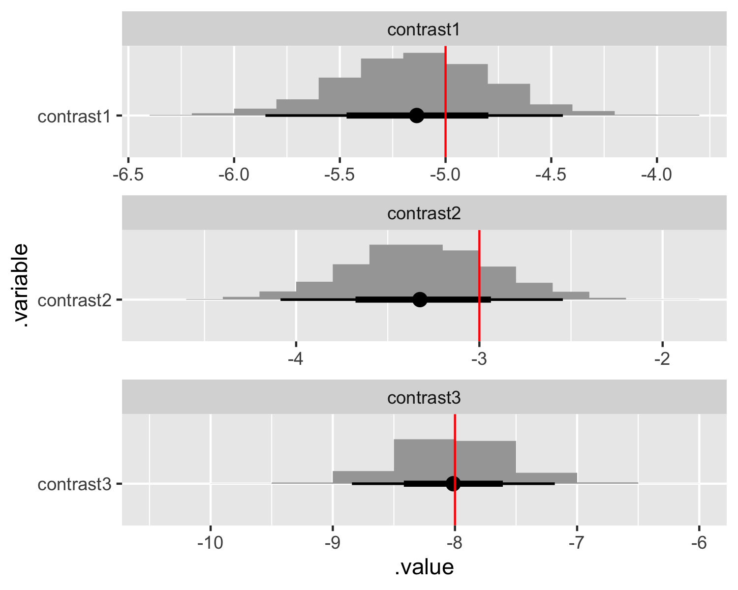
The contrasts and the recovered parameters are the same as the results from the dummy-coded model. Index coding like this is only possible in a Bayesian framework where the use of priors obviates the necessity of strict identification strategies. However, it’s not without costs. We will need to specify informative priors, which we should be doing anyway, and the model itself may take longer to converge.
Final thoughts
Dummy coding is straightforward but requires some care when considering what the reference level and thus the hard-coded contrast should be. For simple models, index coding is great and demonstrates another benefit of being Bayesian. However, for more complicated models or with thinner data, the priors may need to be even more informative to ensure identifiability and model convergence. Finally, you can consider something of a hybrid coding scheme where one of the discrete variables can be index-coded in place of an intercept even when dummy coding with the other discrete variables.